Categorical Variable and Continuous Variable Graph
First off, let's start with what a significant categorical by continuous interaction means. It means that the slope of the continuous variable is different for one or more levels of the categorical variable.
We will use an example from the hsbdemo dataset that has a statistically significant categorical by continuous interaction to illustrate one possible explanatory approach.
The categorical variable is female, a zero/one variable with females coded as one (therefore, male is the reference group). The continuous predictor variable, socst, is a standardized test score for social studies. We will begin by running the regression model and graphing the interaction. Please note that we use c.socst to indicate that socst is a continuous variable.
use https://stats.idre.ucla.edu/stat/data/hsbdemo, clear regress write female##c.socst Source | SS df MS Number of obs = 200 -------------+------------------------------ F( 3, 196) = 49.26 Model | 7685.43528 3 2561.81176 Prob > F = 0.0000 Residual | 10193.4397 196 52.0073455 R-squared = 0.4299 -------------+------------------------------ Adj R-squared = 0.4211 Total | 17878.875 199 89.843593 Root MSE = 7.2116 ------------------------------------------------------------------------------ write | Coef. Std. Err. t P>|t| [95% Conf. Interval] -------------+---------------------------------------------------------------- 1.female | 15.00001 5.09795 2.94 0.004 4.946132 25.05389 socst | .6247968 .0670709 9.32 0.000 .4925236 .7570701 | female#| c.socst | 1 | -.2047288 .0953726 -2.15 0.033 -.3928171 -.0166405 | _cons | 17.7619 3.554993 5.00 0.000 10.75095 24.77284 ------------------------------------------------------------------------------ twoway (scatter write socst, msym(oh) jitter(3)) /// (lfit write socst if ~female)(lfit write socst if female), /// legend(order(2 "male" 3 "female"))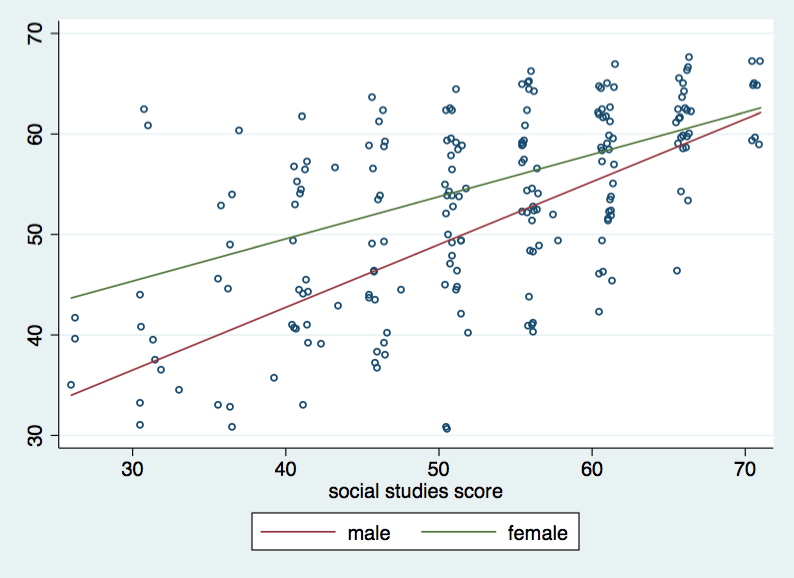
Looking at the graph, we can see that the two regression lines are not parallel and that the line for females falls above the line for males. How could we tell that females are higher than males? The coefficient for female is positive (15.00) which tells us that the level for females is higher than for males.
Let's interpret the coefficients for this model starting with the constant (17.76). This is the value of the intercept for socst regressed on write for males. i.e., the expected value for write when both socst and female equal zero.
The coefficient for socst is .6247 which is the slope of the regression line for the male group (i.e., female=0). The value for the female by socst interaction is -.2047 which is the difference in slope between the male and female group, i.e., the slope for the female group would be about .6248 – .2047 = .4201.
We can also get the slopes for the two groups using the margins command.
margins female, dydx(socst) Average marginal effects Number of obs = 200 Model VCE : OLS Expression : Linear prediction, predict() dy/dx w.r.t. : socst ------------------------------------------------------------------------------ | Delta-method | dy/dx Std. Err. z P>|z| [95% Conf. Interval] -------------+---------------------------------------------------------------- socst | female | 0 | .6247968 .0670709 9.32 0.000 .4933403 .7562533 1 | .420068 .0678044 6.20 0.000 .2871739 .5529622 ------------------------------------------------------------------------------
The difference between males and females may or may not be significantly different for different values of socst. What we will do is look at the male-female difference for various values of socst using the margins command. We will let socst vary between 25 and 70 in increments of 5.
margins, at(female=(0 1) socst=(25(5)70)) vsquish Adjusted predictions Number of obs = 200 Model VCE : OLS Expression : Linear prediction, predict() 1._at : female = 0 socst = 25 2._at : female = 0 socst = 30 3._at : female = 0 socst = 35 4._at : female = 0 socst = 40 5._at : female = 0 socst = 45 6._at : female = 0 socst = 50 7._at : female = 0 socst = 55 8._at : female = 0 socst = 60 9._at : female = 0 socst = 65 10._at : female = 0 socst = 70 11._at : female = 1 socst = 25 12._at : female = 1 socst = 30 13._at : female = 1 socst = 35 14._at : female = 1 socst = 40 15._at : female = 1 socst = 45 16._at : female = 1 socst = 50 17._at : female = 1 socst = 55 18._at : female = 1 socst = 60 19._at : female = 1 socst = 65 20._at : female = 1 socst = 70 ------------------------------------------------------------------------------ | Delta-method | Margin Std. Err. z P>|z| [95% Conf. Interval] -------------+---------------------------------------------------------------- _at | 1 | 33.38182 1.94946 17.12 0.000 29.56095 37.20269 2 | 36.5058 1.645495 22.19 0.000 33.28069 39.73091 3 | 39.62979 1.356406 29.22 0.000 36.97128 42.28829 4 | 42.75377 1.094051 39.08 0.000 40.60947 44.89807 5 | 45.87775 .8825999 51.98 0.000 44.14789 47.60762 6 | 49.00174 .7654688 64.02 0.000 47.50145 50.50203 7 | 52.12572 .78602 66.32 0.000 50.58515 53.66629 8 | 55.24971 .9352206 59.08 0.000 53.41671 57.0827 9 | 58.37369 1.164634 50.12 0.000 56.09105 60.65633 10 | 61.49767 1.436326 42.82 0.000 58.68253 64.31282 11 | 43.26361 2.015017 21.47 0.000 39.31425 47.21297 12 | 45.36395 1.700513 26.68 0.000 42.031 48.69689 13 | 47.46429 1.397521 33.96 0.000 44.72519 50.20338 14 | 49.56463 1.115464 44.43 0.000 47.37836 51.75089 15 | 51.66497 .8748286 59.06 0.000 49.95033 53.3796 16 | 53.76531 .7185139 74.83 0.000 52.35704 55.17357 17 | 55.86565 .7050327 79.24 0.000 54.48381 57.24748 18 | 57.96599 .8412798 68.90 0.000 56.31711 59.61486 19 | 60.06633 1.071589 56.05 0.000 57.96605 62.1666 20 | 62.16667 1.348602 46.10 0.000 59.52346 64.80988 ------------------------------------------------------------------------------
So, the write value for males at socst = 25 is 33.38182 as shown in row 1. The same value for females is 43.26361 as shown in row 11. Here is the differences in the two values, 43.26361 – 33.38182 = 9.88179. We can obtain this difference for all of the values of socst using the margins command with the dydx option.
margins, dydx(female) at(socst=(25(5)70)) vsquish Conditional marginal effects Number of obs = 200 Model VCE : OLS Expression : Linear prediction, predict() dy/dx w.r.t. : 1.female 1._at : socst = 25 2._at : socst = 30 3._at : socst = 35 4._at : socst = 40 5._at : socst = 45 6._at : socst = 50 7._at : socst = 55 8._at : socst = 60 9._at : socst = 65 10._at : socst = 70 ------------------------------------------------------------------------------ | Delta-method | dy/dx Std. Err. z P>|z| [95% Conf. Interval] -------------+---------------------------------------------------------------- 1.female | _at | 1 | 9.881789 2.803692 3.52 0.000 4.386654 15.37692 2 | 8.858145 2.366305 3.74 0.000 4.220273 13.49602 3 | 7.834501 1.947538 4.02 0.000 4.017396 11.6516 4 | 6.810857 1.562436 4.36 0.000 3.748538 9.873176 5 | 5.787213 1.242702 4.66 0.000 3.351562 8.222863 6 | 4.763569 1.049859 4.54 0.000 2.705882 6.821255 7 | 3.739925 1.055888 3.54 0.000 1.670423 5.809426 8 | 2.716281 1.257931 2.16 0.031 .250782 5.181779 9 | 1.692637 1.582617 1.07 0.285 -1.409236 4.794509 10 | .6689926 1.970219 0.34 0.734 -3.192565 4.53055 ------------------------------------------------------------------------------ Note: dy/dx for factor levels is the discrete change from the base level.
Now, we can graph these differences using the marginsplot command.
marginsplot, yline(0)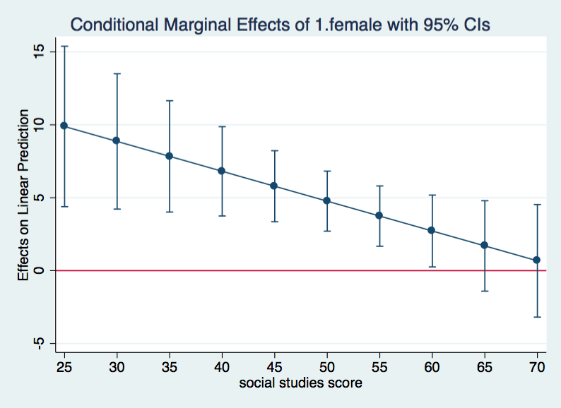
We can see that the differences between males and females is significant for values of socst below about 60. This graph is nice and tells the story we want to know but it is not the best looking graph we can draw. By recasting the lines and confidence intervals we get a much sharper looking graph.
marginsplot, recast(line) recastci(rarea) yline(0)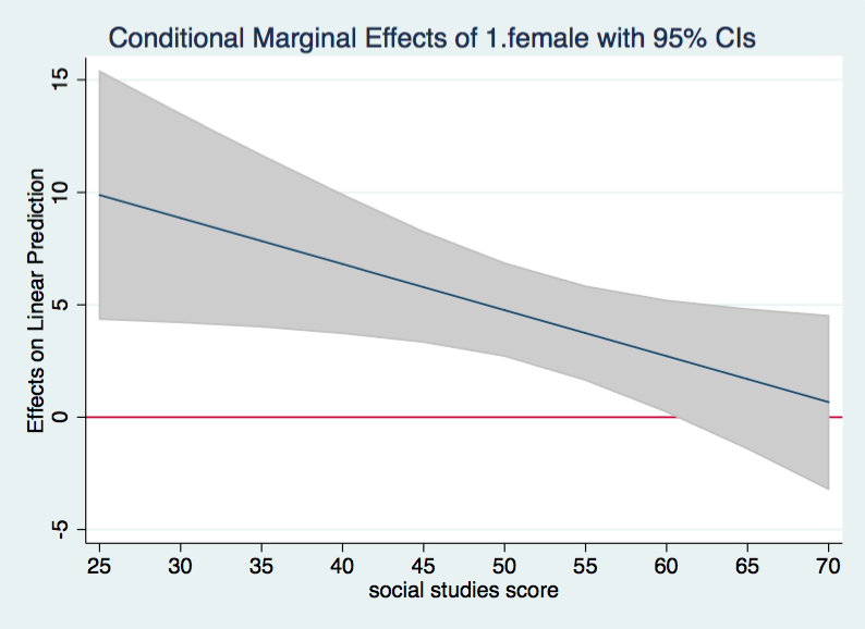
Ah, that's much better.
The graph shows that the male/female differences decreases as the value of socst increases. Whenever the 95% confidence interval for the difference does not include zero, the difference can be considered to be statistically significant. This looks to be the case for all values of socst up to about 60. For socst values greater than 60 the males/female difference is not significant.
A three level categorical variable
What if your categorical variable has more than two levels? The dataset catcon3l has a categorical predictor, b, with three levels. The response variable is y, the categorical predictor is b and it is interacted with a continuous predictor x, specified in Stata as c.x.
use https://stats.idre.ucla.edu/stat/data/catcon3l, clear regress y b##c.x Source | SS df MS Number of obs = 200 -------------+------------------------------ F( 5, 194) = 32.02 Model | 8083.95798 5 1616.7916 Prob > F = 0.0000 Residual | 9794.91702 194 50.489263 R-squared = 0.4522 -------------+------------------------------ Adj R-squared = 0.4380 Total | 17878.875 199 89.843593 Root MSE = 7.1056 ------------------------------------------------------------------------------ y | Coef. Std. Err. t P>|t| [95% Conf. Interval] -------------+---------------------------------------------------------------- b | 2 | -14.56722 7.178201 -2.03 0.044 -28.72455 -.4098837 3 | -20.16644 6.779483 -2.97 0.003 -33.53739 -6.795485 | x | .2728512 .086295 3.16 0.002 .1026544 .4430479 | b#c.x | 2 | .1349579 .1453856 0.93 0.354 -.1517813 .4216972 3 | .3012428 .1203257 2.50 0.013 .0639282 .5385573 | _cons | 42.03102 4.907897 8.56 0.000 32.35134 51.71071 ------------------------------------------------------------------------------ /* test of overall significant of the interaction */ testparm b#c.x ( 1) 2.b#c.x = 0 ( 2) 3.b#c.x = 0 F( 2, 194) = 3.15 Prob > F = 0.0453 /* or */ contrast b#c.x Contrasts of marginal linear predictions Margins : asbalanced ------------------------------------------------ | df F P>F -------------+---------------------------------- b#c.x | 2 3.15 0.0453 | Residual | 194 ------------------------------------------------
The testparm and/or contrast commands show that the overall interaction is statistically significant.
Next, we will compute the simple slopes using the margins command.
margins b, dydx(x) Average marginal effects Number of obs = 200 Model VCE : OLS Expression : Linear prediction, predict() dy/dx w.r.t. : x ------------------------------------------------------------------------------ | Delta-method | dy/dx Std. Err. z P>|z| [95% Conf. Interval] -------------+---------------------------------------------------------------- x | b | 1 | .2728512 .086295 3.16 0.002 .1037161 .4419862 2 | .4078091 .1170049 3.49 0.000 .1784837 .6371345 3 | .5740939 .0838538 6.85 0.000 .4097435 .7384444 ------------------------------------------------------------------------------
The slope for b = 1 seems to be different from the slopes of b equal 2 or 3.
Now, let's graph the slopes along with a scatterplot of the data. We will do this by quietly running margins (to suppress the large output) followed by a marginsplot command with added scatterplot.
quietly margins b, at(x=(25(5)70)) marginsplot, recast(line) noci addplot(scatter y x, jitter(3) msym(oh))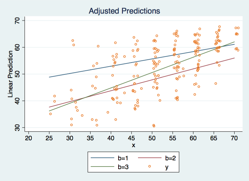
Let's see if the slope for b = 3 is significantly different from each of the other two slopes. We will test this using reference contrasts with the margins command. We will indicate that slope 3 is the reference using b3 and reference group coding with r which combine to rb3.
margins rb3.b, dydx(x) margins rb3.b, dydx(x) Contrasts of average marginal effects Model VCE : OLS Expression : Linear prediction, predict() dy/dx w.r.t. : x ------------------------------------------------ | df chi2 P>chi2 -------------+---------------------------------- x | b | (1 vs 3) | 1 6.27 0.0123 (2 vs 3) | 1 1.33 0.2480 Joint | 2 6.29 0.0430 ------------------------------------------------ -------------------------------------------------------------- | Contrast Delta-method | dy/dx Std. Err. [95% Conf. Interval] -------------+------------------------------------------------ x | b | (1 vs 3) | -.3012428 .1203257 -.5370769 -.0654086 (2 vs 3) | -.1662848 .14395 -.4484217 .115852 --------------------------------------------------------------
We see that slope 3 is significantly different from slope 1 but is not different from slope 2.
Looking at the three slopes one might wonder where the differences between groups are statistically significant. The most natural way to do this is to pick a reference group, this time b = 1 and see where the values for b = 2 are different and then the same for b1 versus b3. Again, the margins command with the dydx option comes to mind.
margins, dydx(b) at(x=(25(5)70)) vsquish Conditional marginal effects Number of obs = 200 Model VCE : OLS Expression : Linear prediction, predict() dy/dx w.r.t. : 2.b 3.b 1._at : x = 25 2._at : x = 30 3._at : x = 35 4._at : x = 40 5._at : x = 45 6._at : x = 50 7._at : x = 55 8._at : x = 60 9._at : x = 65 10._at : x = 70 ------------------------------------------------------------------------------ | Delta-method | dy/dx Std. Err. z P>|z| [95% Conf. Interval] -------------+---------------------------------------------------------------- 2.b | _at | 1 | -11.19327 3.704771 -3.02 0.003 -18.45448 -3.93205 2 | -10.51848 3.055425 -3.44 0.001 -16.507 -4.529954 3 | -9.843688 2.450055 -4.02 0.000 -14.64571 -5.041668 4 | -9.168898 1.930483 -4.75 0.000 -12.95258 -5.385221 5 | -8.494108 1.583543 -5.36 0.000 -11.59779 -5.390422 6 | -7.819319 1.531437 -5.11 0.000 -10.82088 -4.817758 7 | -7.144529 1.799955 -3.97 0.000 -10.67238 -3.616682 8 | -6.469739 2.278427 -2.84 0.005 -10.93537 -2.004105 9 | -5.79495 2.863471 -2.02 0.043 -11.40725 -.1826503 10 | -5.12016 3.502078 -1.46 0.144 -11.98411 1.743787 -------------+---------------------------------------------------------------- 3.b | _at | 1 | -12.63537 3.853374 -3.28 0.001 -20.18784 -5.082896 2 | -11.12916 3.285978 -3.39 0.001 -17.56956 -4.688757 3 | -9.622942 2.733264 -3.52 0.000 -14.98004 -4.265844 4 | -8.116729 2.206291 -3.68 0.000 -12.44098 -3.792477 5 | -6.610515 1.728765 -3.82 0.000 -9.998831 -3.222199 6 | -5.104301 1.354048 -3.77 0.000 -7.758187 -2.450415 7 | -3.598087 1.184137 -3.04 0.002 -5.918953 -1.277221 8 | -2.091873 1.301856 -1.61 0.108 -4.643464 .4597175 9 | -.5856595 1.64663 -0.36 0.722 -3.812996 2.641677 10 | .9205543 2.109945 0.44 0.663 -3.214862 5.055971 ------------------------------------------------------------------------------ Note: dy/dx for factor levels is the discrete change from the base level.
The first block of results, 2.b compares b1 with b2 and are significant for x values less thatn 70. The second block, b3 compares b1 with b3 and are significant for x values less thatn 60. Let's graph these margins results.
marginsplot, recast(line) recastci(rarea) yline(0)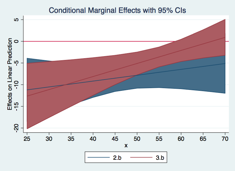
The blue shaded area is b1 vs b2 while the red shaded area is b1 vs b3. The graph reaffirms our interpretation of the margins table.
Source: https://stats.oarc.ucla.edu/stata/faq/how-can-i-understand-a-categorical-by-continuous-interaction-stata-12/
0 Response to "Categorical Variable and Continuous Variable Graph"
Postar um comentário